To Fake or Not to Fake
What do you call a library full of fake news?
A lie-brary.
Intro
Fake news has become a hot topic in the United States and the world in the past decade, accelerated by rising popularity of the internet and the ease of creating and sharing information, especially on platforms that may not regulate information that is being passed through them. As a consumer of the news, one must be vigilant of what they are reading and critically think about the information they are being given. Today, we are going to take a look on how to build our own machine learning model using tensorflow and keras to identify fake news. Using article titles and article text, we are going to determine what model performs the best in terms of classifying fake news accurately.
📰1
As always, lets import our libaries and modules! Addtionally, lets run the code to extract the data we will be working with today and seperate them into useful datasets.
import numpy as np
import pandas as pd
import tensorflow as tf
import re
import string

from tensorflow.keras import layers, losses, Input, Model, utils
from tensorflow.keras.layers.experimental.preprocessing import TextVectorization, StringLookup

from sklearn.model_selection import train_test_split
from sklearn.preprocessing import LabelEncoder
from sklearn.decomposition import PCA

# for embedding viz
import matplotlib.pyplot as plt

import plotly.express as px
import plotly.io as pio
pio.templates.default = "plotly_white"

# for stopwords
import nltk
nltk.download('stopwords') #run once per kernal restart

# import training data
train_url = "https://github.com/PhilChodrow/PIC16b/blob/master/datasets/fake_news_train.csv?raw=true"
df = pd.read_csv(train_url, index_col = 0)
📰2
Now, lets create some dataset creation functions to take our dataframe and convert them into tensors for our machine learning models to process!
from gensim.utils import simple_preprocess # lowercases, tokenizes, de-accents
from nltk.corpus import stopwords
stop_words = stopwords.words('english')

def remove_stopwords(texts):
  return [' '.join([word for word in simple_preprocess(str(doc)) if word not in stop_words]) for doc in texts]

def make_dataset(data):
  # preprocess the dataset for feeding into the tensorflow model
  data['title'] = remove_stopwords(data['title']) #remove stopwords from titles
  data['text'] = remove_stopwords(data['text']) #remove stopwords from text
  data = tf.data.Dataset.from_tensor_slices( #process it into a tensorflow data
      (
        {
            "title" : data[["title"]],
            "text" : data[["text"]]
        },
        {
            "fake" : data["fake"]
        }
    )
  )
  return data.batch(100)
Now lets create our dataset, and split it into train, test, and validation.
data = make_dataset(df)

train_size = int(0.7*len(data))
val_size = int(0.2*len(data))

train = data.take(train_size)
val = data.skip(train_size).take(val_size) # data[train_size : train_size + val_size]
test = data.skip(train_size+val_size) #  data[train_size + val_size:]
Awesome! Now that our data is split and in the right format, lets find out what the base rate of our machine learning models should be.
labels_iterator= train.unbatch().map(lambda text, fake: fake).as_numpy_iterator()

fake = 0
not_fake = 0

for labels in (labels_iterator):
  value = labels['fake']
  if value == 1:
      fake += 1
  else:
      not_fake += 1

fake, not_fake
(8217, 7483)
As shown, the sample is slightly skewed towards the not_fake label, such that only 47.66% of the labels are not_fake, while the other 52.34% are fake. Therefore our baseline model will predict that an article is fake 52.34% of the time.
📰3
Lets start making our models!
Model 1
In model 1, we are going to use the title of articles only as our features to classify if an article is fake news or not.
As part of our classification problem, we must first convert our words into numbers using text vectorization and filtering.
#preparing a text vectorization layer for tf model
size_vocabulary = 2000

def standardization(input_data):
    lowercase = tf.strings.lower(input_data)
    no_punctuation = tf.strings.regex_replace(lowercase,
                                  '[%s]' % re.escape(string.punctuation),'')
    return no_punctuation

title_vectorize_layer = TextVectorization(
    standardize=standardization,
    max_tokens = size_vocabulary, # only consider this many words
    output_mode='int',
    output_sequence_length=500)

title_vectorize_layer.adapt(train.map(lambda x, y: x["title"])) #now the title_vectorize_layer knows to do the title !

titles_input = Input(
    shape = (1,),
    name = "title",
    dtype = "string"
)

title_features = title_vectorize_layer(titles_input) # apply the vectorization layer to the titles_input
title_features = layers.Embedding(size_vocabulary, output_dim = 3, name="embedding_title")(title_features)
title_features = layers.Dropout(0.2)(title_features)
title_features = layers.GlobalAveragePooling1D()(title_features)
title_features = layers.Dropout(0.2)(title_features)
title_features = layers.Dense(32, activation='relu')(title_features)
output = layers.Dense(2, name = "fake")(title_features)

model1 = Model(
    inputs = titles_input,
    outputs = output
)
Now that our model has been created and our data has been cleaned. We can now fit our model to our training set and evaluate its performance on the validation set.
model1.compile(optimizer="adam",
              loss = losses.SparseCategoricalCrossentropy(from_logits=True),
              metrics=["accuracy"])

history = model1.fit(train,
                    validation_data=val,
                    epochs = 50,
                    verbose = False)

plt.plot(history.history["accuracy"], label = "training")
plt.plot(history.history["val_accuracy"], label = "validation")
plt.gca().set(xlabel = "epoch", ylabel = "accuracy")
plt.legend()
plt.show()
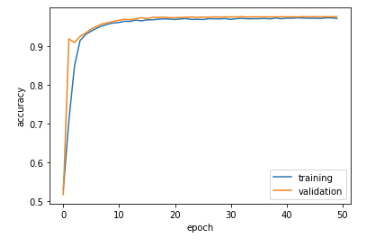
Wow! Model1 is preforming super well, coming out with a validation accuracy of 0.9764 at the 50th epoch.
Model 2
In model 2, we are going to be doing a similar process as in model 1, but using article text instead of title as our feature. Let’s see how much better or worse our text model does in comparison to our title model!
text_vectorize_layer = TextVectorization(
    standardize=standardization,
    max_tokens=size_vocabulary, # only consider this many words
    output_mode='int',
    output_sequence_length=500)

text_vectorize_layer.adapt(train.map(lambda x, y: x["text"])) #now the text_vectorize_layer knows to do the text !

text_input = Input(
    shape = (1,),
    name = "text",
    dtype = "string"
)

text_features = text_vectorize_layer(text_input) # apply the vectorization layer to the titles_input
text_features = layers.Embedding(size_vocabulary, output_dim = 7, name="embedding_text")(text_features)
text_features = layers.Dropout(0.2)(text_features)
text_features = layers.GlobalAveragePooling1D()(text_features)
text_features = layers.Dropout(0.2)(text_features)
text_features = layers.Dense(32, activation='relu')(text_features)
output = layers.Dense(2, name = "fake")(text_features)

model2 = Model(
    inputs = text_input,
    outputs = output
)
Now that our model has been created and our data has been cleaned. We can now fit our model to our training set and evaluate its performance on the validation set.
model2.compile(optimizer="adam",
              loss = losses.SparseCategoricalCrossentropy(from_logits=True),
              metrics=["accuracy"])

history = model2.fit(train,
                    validation_data=val,
                    epochs = 50,
                    verbose = False)

plt.plot(history.history["accuracy"], label = "training")
plt.plot(history.history["val_accuracy"], label = "validation")
plt.gca().set(xlabel = "epoch", ylabel = "accuracy")
plt.legend()
plt.show()
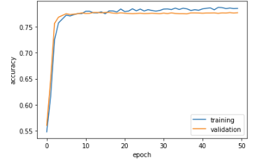
Interesting!!! It seems that our second model performs much worse than our first model in terms of validation accuracy, coming out at a solid 0.7767 at the 50th epoch. Let’s see if a combination of model 1 and model 2 can yield a high accuracy model.
Model 3
Like models 1 and 2, we need to create the layers in our model and process our data. Because we are using the same layers found in model 1 and model 2, we can call it in our functional api!
title_features = title_features
text_features = text_features
main = layers.concatenate([title_features, text_features], axis = 1)
main = layers.Dense(32, activation='relu')(main)
output = layers.Dense(2, name="fake")(main)

model3 = Model(
    inputs = [titles_input, text_input],
    outputs = output
)

model3.compile(optimizer="adam",
              loss = losses.SparseCategoricalCrossentropy(from_logits=True),
              metrics=["accuracy"])

history = model3.fit(train,
                    validation_data=val,
                    epochs = 50,
                    verbose = False)

plt.plot(history.history["accuracy"], label = "training")
plt.plot(history.history["val_accuracy"], label = "validation")
plt.gca().set(xlabel = "epoch", ylabel = "accuracy")
plt.legend()
plt.show()
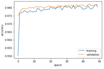
How intriguing! Model 3 acts like model 1, which exclusively looked at article title alone, such that the accuracies of training and validation are quite high. Coming out at a solid 0.9815 at the 50th epoch, the model is able to classify fake news at a higher level than model 1.
Given this, we know that model 3 has the best odds at predicting whether an article is truly fake news or not. Lets evaluate our model with some test data!
📰4
Lets import our test set and score our model!
test_url = "https://github.com/PhilChodrow/PIC16b/blob/master/datasets/fake_news_test.csv?raw=true" #import test data
test_pd = pd.read_csv(train_url, index_col = 0)
test_data = make_dataset(test_pd)

model3.evaluate(test_data)
225/225 [==============================] - 8s 37ms/step - loss: 0.0477 - accuracy: 0.9849
Amazing! Our model still performs at a high level when faced with novel data. As seen from the above tests, using a combination of article titles and article text as features to determine if an article is fake news is an effective strategy.
📰5
Alright! Now that we know how our models work, lets take a closer look at our embedding process to understand how we go from words to numbers!
weights = model1.get_layer('embedding_title').get_weights()[0]# get the weights from the embedding_title layer
vocab = title_vectorize_layer.get_vocabulary()                # get the vocabulary from our data prep for later

pca = PCA(n_components=3)
weights = pca.fit_transform(weights)
x0 = weights[:,0]
x1 = weights[:,1]
x2 = weights[:,2]

embedding_df = pd.DataFrame({
    'word' : vocab,
    'x0'   : x0,
    'x1'   : x1,
    'x2' : x2
})


fig = px.scatter(embedding_df,
                 x = "x0",
                 y = "x1",
                 size = [2]*len(embedding_df),
                # size_max = 2,
                 hover_name = "word")

fig.show()
Wow thats so cool! As you can see the majority of the words are clustered up in the middle. There are a few distinct words I would like to highlight of interest. The rightmost point is “video” while the leftmost point is “factbox”. Factbox is a term used in headlines to describe the article which contains a lot of “facts”, and not much opinion. (see https://www.usnews.com/news/technology/articles/2022-05-12/factbox-u-s-companies-and-their-cryptocurrency-holdings for an example.) It seems that a compelling difference between two articles and the way they are vectorized in our model would be if they include either factbox or video in the title.
Additionally, looking in the right side of the plot you can find: Hillary, GOP, and Breaking. They are all relatively close together, but still far away from the central horde of plots. Like factbox and video, we can interpret that these words also have a large impact on classification of fake news by our model. Its been known that the elections in the past few years has been controversal, especially with the proliferation of fake news. It makes sense that bait words such as breaking are associated with Hillary and GOP, often the subjects of the news headline.
Thank you for reading! See you again soon ^.^


