Cat or Dog
What do you call a storm that’s raining cats and dogs?
A furricane.
Intro
Machine Learning has become a hot topic in recent years, everyone wants to be able to utilize this powerful tool in their individual enterprises. Today, we are going to take a look on how to build our own machine learning model using tensorflow and keras. Using our newly aqcuired skills, we can the appropriate changes to our model to create one that can accurately identify dogs and cats based on image alone. With this image classification problem, we can use further use transfer learning to achieve our goals.
🐈1
As always, lets import our libaries and modules! Addtionally, lets run the code to extract the data we will be working with today and seperate them into useful datasets.
import os
from tensorflow.keras import utils
import tensorflow as tf
import tensorflow.keras as keras
import numpy as np
import matplotlib.pyplot as plt

# location of data
_URL = 'https://storage.googleapis.com/mledu-datasets/cats_and_dogs_filtered.zip'

# download the data and extract it
path_to_zip = utils.get_file('cats_and_dogs.zip', origin=_URL, extract=True)

# construct paths
PATH = os.path.join(os.path.dirname(path_to_zip), 'cats_and_dogs_filtered')

train_dir = os.path.join(PATH, 'train')
validation_dir = os.path.join(PATH, 'validation')

# parameters for datasets
BATCH_SIZE = 32
IMG_SIZE = (160, 160)

# construct train and validation datasets
train_dataset = utils.image_dataset_from_directory(train_dir,
                                                   shuffle=True,
                                                   batch_size=BATCH_SIZE,
                                                   image_size=IMG_SIZE)

validation_dataset = utils.image_dataset_from_directory(validation_dir,
                                                        shuffle=True,
                                                        batch_size=BATCH_SIZE,
                                                        image_size=IMG_SIZE)

# construct the test dataset by taking every 5th observation out of the validation dataset
val_batches = tf.data.experimental.cardinality(validation_dataset)
test_dataset = validation_dataset.take(val_batches // 5)
validation_dataset = validation_dataset.skip(val_batches // 5)


AUTOTUNE = tf.data.AUTOTUNE
train_dataset = train_dataset.prefetch(buffer_size=AUTOTUNE)
validation_dataset = validation_dataset.prefetch(buffer_size=AUTOTUNE)
test_dataset = test_dataset.prefetch(buffer_size=AUTOTUNE)
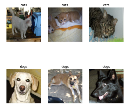
By now, we should have 3 datasets (train, validation, and test) which we can use to train our machine learning model and eventually evaluate it on our test data. Let’s take a look at some of our train data so we have a better understanding of what data we are working with.
def cat_dog_maker():
    images, labels = list(train_dataset.take(1))[0]

    plt.figure(figsize=(8, 8))
    #cats
    for i in range(3):
      ax = plt.subplot(2,3, i+1)
      index = np.where(labels == 0)[0][i]
      plt.imshow(images[index].numpy().astype("uint8"))
      plt.title("cats")
      plt.axis("off")

    #dogs
    for i in range(3):
      ax = plt.subplot(2,3, i+4)
      index = np.where(labels == 1)[0][i]
      plt.imshow(images[index].numpy().astype("uint8"))
      plt.title("dogs")
      plt.axis("off")

    plt.show()

#call function
cat_dog_maker()
Wow! From our graph we can see that our data is split into photos of various cats and dogs. Lets get a better look at our entire training dataset.
labels_iterator= train_dataset.unbatch().map(lambda image, label: label).as_numpy_iterator()

cats = 0
dogs = 0

for labels in labels_iterator:
  if labels == 0:
    cats += 1
  else:
    dogs +=1

cats, dogs
(1000, 1000)
From our label_iterator, we were able to extract the labels of our dataset, which are encoded as 0’s and 1’s (representing the two elements of our label class: cat and dog). We can see that there is an equal number of cats and dogs in the train_dataset, whose ratio is also reflective of the entire datasets!
When creating a machine learning model, its oftentimes best to refer to the effectiveness of a model by comparing it to the a baseline machine learning model, which just guesses the most most frequent label in a dataset. For our purposes, since the availibility of cats and dogs in our dataset is the same, we can expect the baseline to have a 50% chance of guessing correctly on our dataset.
🐈2
Now that we have a better understanding of what data we are working with, lets start creating our machine learning model!
model1 = tf.keras.Sequential([
          keras.layers.Conv2D(32, (3, 3), activation='relu', input_shape=(160, 160, 3)),
          keras.layers.MaxPooling2D((2, 2)),
          keras.layers.Conv2D(32, (3, 3), strides = (2,2), activation='relu'),
          keras.layers.MaxPooling2D((2, 2)),
          keras.layers.Conv2D(32, (3, 3), activation='relu'),
          keras.layers.Flatten(), #input to dense must be flattened from 3d -> 1d array
          keras.layers.Dropout(0.2), #hide some neurons
          keras.layers.Dense(64, activation='relu'),
          keras.layers.Dense(2, activation='sigmoid') # number of nodes = classes in your dataset
])

model1.compile(optimizer='adam',
              loss=tf.keras.losses.SparseCategoricalCrossentropy(),
              metrics=['accuracy'])

history = model1.fit(train_dataset,
                     epochs = 20,
                     validation_data= validation_dataset)

#code for plotting our history
#is identical for each model, refer to this code snippet if needed
plt.plot(history.history["accuracy"], label = "training")
plt.plot(history.history["val_accuracy"], label = "validation")
plt.gca().set(xlabel = "epoch", ylabel = "accuracy")
plt.legend()
plt.show()
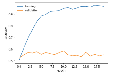
Amazing!!! For our first iteration of our model, we were already able to get a consistent 54-55% validation accuracy on our validation dataset! Compared to our baseline model, we are slightly more accurate but not by a large margin. In terms of overfitting, model1 is definetly overfitted because our training accuracy is much higher than our validation accuracy.
🐈3
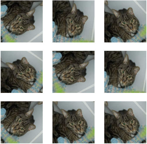
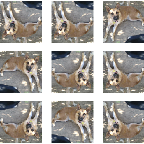
Ok! Now that we are getting into the swing of things for creating and optimizing our model, lets introduce the idea of data augmentation. Data augmentation refers to the practice of including modified copies of the same image in the training set, and by feeding these modified copies into our model, our model will learn how to identify cats and dogs even better!
Lets take a quick look at two data augmentation layers and what they do to images!
plt.figure(figsize=(10, 10))
plt1.figure(figsize=(10, 10))

image = images[1].numpy().astype("uint8")
for i in range(9):
  augmented_image = keras.layers.RandomFlip("horizontal_and_vertical")(image, training = True),
  ax = plt.subplot(3, 3, i + 1)
  plt.imshow(augmented_image[0].numpy().astype("uint8"))
  plt.axis("off")

image = images[5].numpy().astype("uint8")
for i in range(9):
  augmented_image = keras.layers.RandomRotation(0.2)(image, training = True),
  ax = plt1.subplot(3, 3, i + 1)
  plt1.imshow(augmented_image[0].numpy().astype("uint8"))
  plt1.axis("off")
Lets take these layers and throw them into our model!
model2 = tf.keras.Sequential([
          keras.layers.RandomFlip("horizontal_and_vertical"),
          keras.layers.RandomRotation(0.2),
          keras.layers.Conv2D(32, (3, 3), activation='relu', input_shape=(160, 160, 3)),
          keras.layers.MaxPooling2D((2, 2)),
          keras.layers.Conv2D(32, (3, 3), strides = (2,2), activation='relu'),
          keras.layers.MaxPooling2D((2, 2)),
          keras.layers.Conv2D(32, (3, 3), activation='relu'),
          keras.layers.Flatten(), #input to dense must be flattened from 3d -> 1d array
          keras.layers.Dropout(0.2), #hide some neurons
          keras.layers.Dense(64, activation='relu'),
          keras.layers.Dense(2, activation='sigmoid') # number of nodes = classes in your dataset
])

model2.compile(optimizer='adam',
              loss=tf.keras.losses.SparseCategoricalCrossentropy(),
              metrics=['accuracy'])

history = model2.fit(train_dataset,
        epochs = 20,
        validation_data= validation_dataset)
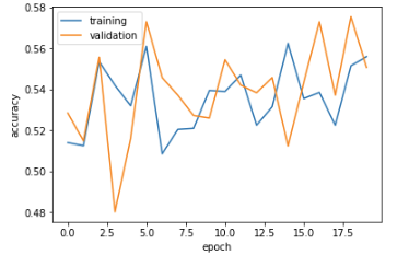
Intriguing!!! Our validation and training accuracy trends are all over the place in comparison to model1. Nevertheless, we can see that the model is hovering somewhat around the 53-56% validation accuracy range. Compared to our accuracy in model1, we are seeing similar outcomes, albeit slightly less consistent in this current model. Unlike model1, model2 does not seem to suffer from any sort of overfitting problems where the validation and training accuracies are similar.
🐈4
Alright! We are making good progress. Now lets add another layer on this cake! We are going to employ a preprocessing layer, which essentially takes our data and normalizes it into more digestable forms for our model to train more efficiently on.
i = tf.keras.Input(shape=(160, 160, 3))
x = tf.keras.applications.mobilenet_v2.preprocess_input(i)
preprocessor = tf.keras.Model(inputs = [i], outputs = [x])

model3 = tf.keras.Sequential([
          preprocessor,
          keras.layers.RandomFlip("horizontal_and_vertical"),
          keras.layers.RandomRotation(0.2),
          keras.layers.Conv2D(32, (3, 3), activation='relu', input_shape=(160, 160, 3)),
          keras.layers.MaxPooling2D((2, 2)),
          keras.layers.Conv2D(64, (3, 3), strides = (2,2), activation='relu'),
          keras.layers.MaxPooling2D((2, 2)),
          keras.layers.Conv2D(32, (3, 3), activation='relu'),
          keras.layers.MaxPooling2D((2, 2)),
          keras.layers.Flatten(), #input to dense must be flattened from 3d -> 1d array
          keras.layers.Dropout(0.2), #hide some neurons
          keras.layers.Dense(64, activation='relu'),
          keras.layers.Dense(2, activation='sigmoid') # number of nodes = classes in your dataset
])

model3.compile(optimizer='adam',
              loss=tf.keras.losses.SparseCategoricalCrossentropy(),
              metrics=['accuracy'])

history = model3.fit(train_dataset,
        epochs = 20,
        validation_data= validation_dataset)
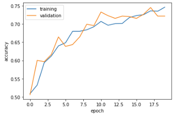
Fantastic!!! Our validation and training accuracy in model3 far surpasses model1 and 2’s. We were able to see a validation accuracy that is consistently hovering around 71-74% accuracy range. Our validation and training accuracy in model3 far surpasses model1 and 2’s, which is awesome! Now that our accuracy has made a significant leap, it is time to consider if we are overfitted our model. All things considered, our model3 is still not at the point in which it is overfitted.
🐈5
Now that we are approaching great and greater models, lets add another layer to ice it off! We are going to use an idea called “TRANSFER LEARNING”, which essentially means that we are going to take a pre-existing model for our identification task.
Firstly, we need to access the base model of this pre-existing model.
IMG_SHAPE = IMG_SIZE + (3,)
base_model = tf.keras.applications.MobileNetV2(input_shape=IMG_SHAPE,
                                               include_top=False,
                                               weights='imagenet')
base_model.trainable = False

i = tf.keras.Input(shape=IMG_SHAPE)
x = base_model(i, training = False)
base_model_layer = tf.keras.Model(inputs = [i], outputs = [x])
Now that our model has been created, lets incorporate it into our main model and see how it preforms!
model4 = tf.keras.Sequential([
          preprocessor,
          keras.layers.RandomFlip("horizontal_and_vertical"),
          keras.layers.RandomRotation(0.2),
          base_model_layer,
          keras.layers.GlobalMaxPooling2D(),
          keras.layers.Dropout(0.2),
          keras.layers.Dense(2, activation='sigmoid') # number of nodes = classes in your dataset
])

model4.compile(optimizer='adam',
              loss=tf.keras.losses.SparseCategoricalCrossentropy(),
              metrics=['accuracy'])

history = model4.fit(train_dataset,
    epochs = 20,
    validation_data = validation_dataset)
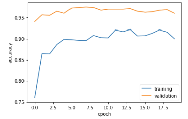
OUTSTANDING!!!!!! We are getting a consistent 96-97% validation accuracy on this model! Compared to our other models, model4 blows everyone in the dust in terms of accuracy. Now, with the insane accuracy of model4 overfitting is a possibility we may consider. With such a high accuracy, there is a real chance that our model4 is too fitted to our dataset due to the small discrepency between validation and training.
🐈6
FANTABULOUS!!!!!!!!!!!!!!!!!!!!!!!!!!!!!!!!!!!!!!!!!!!!!!!!!!!!!!!!!!!!!!!!!! We’ve really explored some important concepts in image classification, but there’s much more to learn.
For now, lets just appreciate the models we’ve created now. Using our best preforming model, model4, lets evaluate how it does against the test dataset!
model4.evaluate(test_dataset)
#6/6 [==============================] - 1s 47ms/step - loss: 0.0992 - accuracy: 0.9688
Amazing! Against our test dataset, model4 still preforms to standard, obtaining a 96.88% accuracy on the images. Woohoo! That’s something to celebrate.
That’s it for today folks. Go enjoy the rest of your day and thanks for reading!

